[notes] Inferring Change Points in High-Dimensional Linear Regression via Approximate Message Passing

This paper aims to address the problem of localizing change points in high-dimensional linear regression. Their major contribution is to put forward an Approximate Message Passing algorithm for estimating signals and changing point locations.

What is it and why it is important?

How does it exploit prior information on signal noise and change points? More specifically, how to compute the approximate posterior distribution?

These are the questions raised in my mind when I start reading and I’ll go through the essay to find the answers.

Background intro

Heterogeneity in high-dimensional datasets

Heterogeneity means that the regression parameters are not constant across the data, but vary depending on some factors. When the data are ordered by time, a simple form of heterogeneity is a change in the data-generating mechanism at certain unknown instants of time. If these ‘change points’ were known, or estimated accurately, the dataset could be partitioned into homogeneous subsets, each amenable to analysis via standard statistical techniques (Fryzlewicz, 2014).

Models with change points overview

In a variety of fields including genomics, neuroscience, and economics, the detection of changes is studied with the following statistical contexts:

1. signal means (Wang & Samworth, 2018; Wang et al., 2020; Liu et al., 2021);
2. covariance structures (Cho & Fryzlewicz, 2015; Wang et al., 2021b);
3. graphs (Londschien et al., 2023; Bhattacharjee et al., 2020; Fan & Guan, 2018);
4. dynamic networks (Wang et al., 2021a); and functionals (Madrid Padilla et al., 2022).

Change points in High-dimensional Linear Regression

Concepts

1. Change points: The sample indices where regression vector $\beta^{(i)}$ changes. (We set the number of change points to be $L^*-1$)
2. Distinct signals: The distinct straight lines in the $\beta^{(i)}$s sequence. (We set the number of distinct signals to be $L^*$, with the upper bound $L$)

goal: estimate change point location and $L*$, also quantify uncertainty via confidence set or posterior distribution.

Recent works

1. Sparse: Most of these papers consider the setting where the signals are sparse and analyze procedures that combine the LASSO estimator (or a variant) with a partitioning technique, e.g., dynamic programming. However, incorporating sparsity-based constraints cannot be easily adapted to take advantage of other types of signal priors.

2. Bayesian: Bayesian approaches to change point detection have been studied in several works, however, they mainly focus on (low-dimensional) time series.

Authors claim their method is especially good at exploiting prior information on the change point locations, which the above works can hardly do. What is that prior information and how much can we gain from it?

Describe change points

The model’s ideas can be straightforward, but it’s a subtle work to encode them into formal mathematical language and be cautious to avoid exceptional cases slipping through the cracks.

Here are some notes I took down while reading this paper. (I feel that they are helpful for both understanding AMP and learning to deliver complex system.)

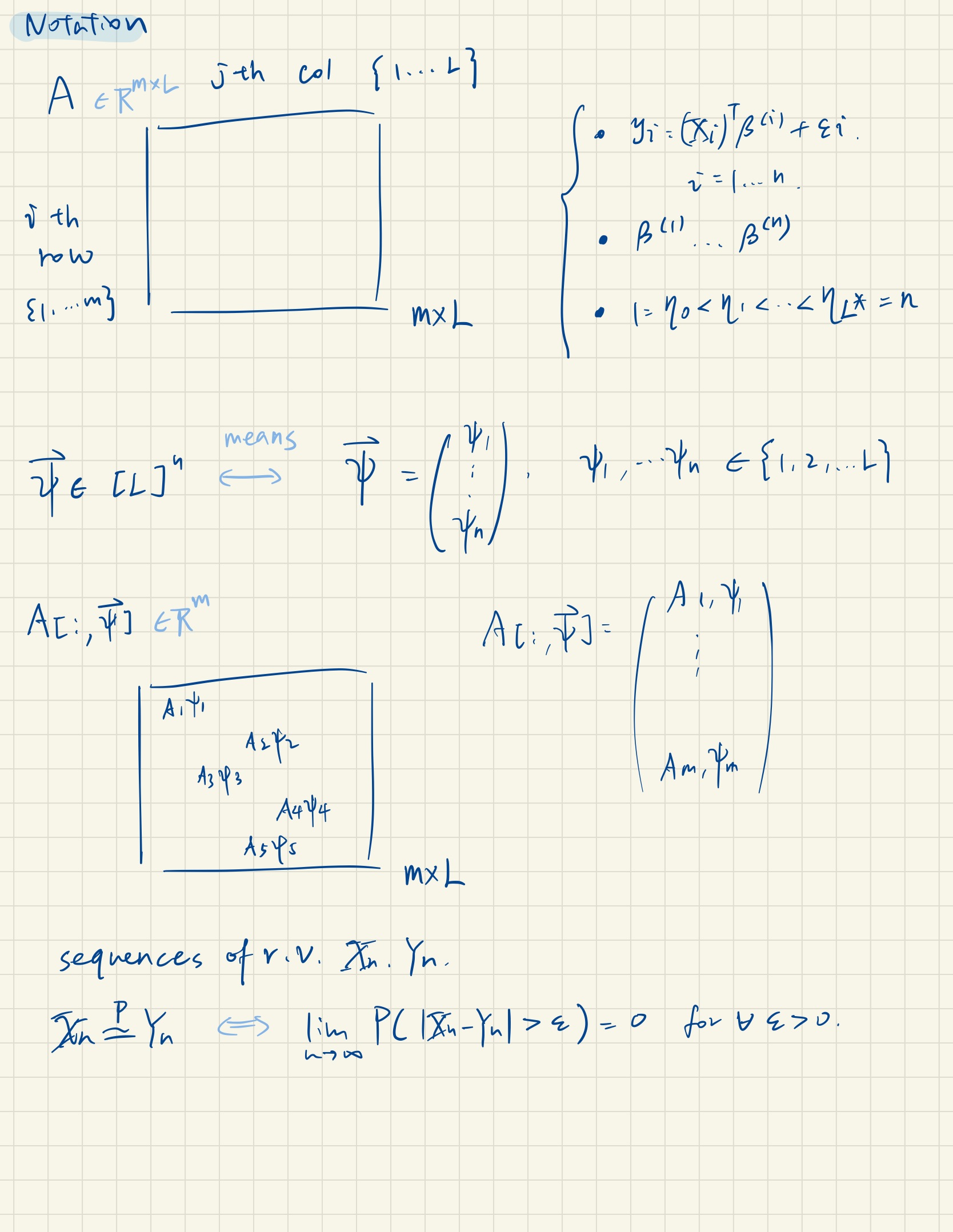
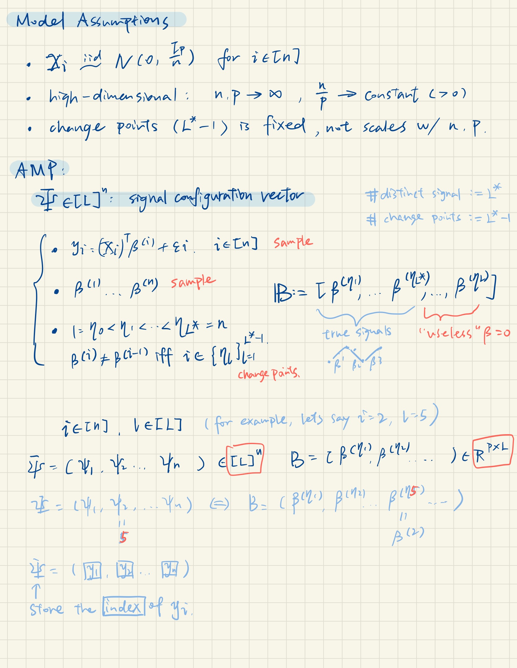
Note that [] is a set with sequence {1,2,….L}, so $ \phi[L]^n$ is a vector where each element in the vector belongs to that set separately.

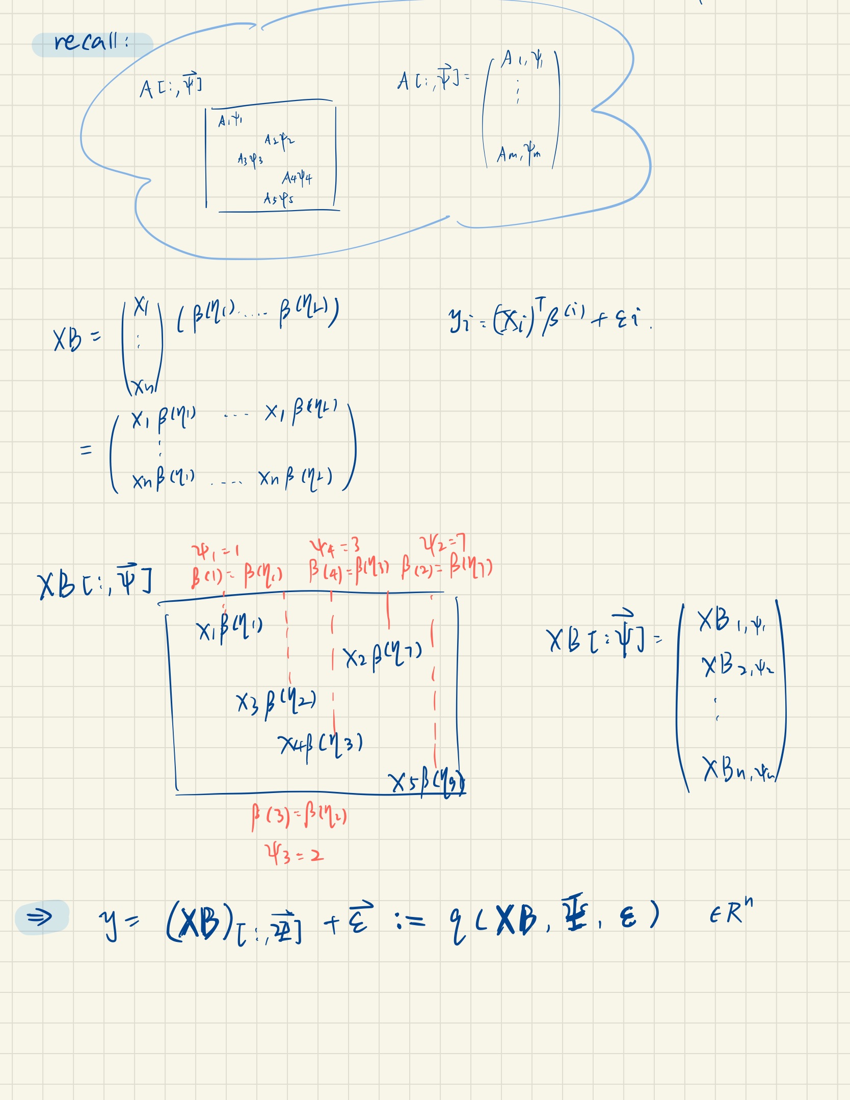
So the goal of the AMP algorithm is to estimate the signal matrix $B$ and true change points in $\eta$.

AMP as an iteration method

That’s the part I spent the longest time on… Since I’m not familiar with this kind of iteration algorithm, I started with the Jacobi and Gauss-Seidel Iterative Methods to understand the innovation of AMP.

In each iteration $t \ge 1$, AMP produces an updated estimate of the signal matrix $B$, which we call $B^t$, and of the linearly transformed signal $\Theta:=XB$, which we call $\Theta^t$. These estimates have distributions that can be described by a deterministic low-dimensional matrix recursion called \textit{state evolution}.

Starting with an initializer $B^0\in R^{p\times L}$ and defining $\hat{R}^{-1}:=0_{n\times L}, $ for $t \geq 0$ the algorithm computes: %% \begin{align} \begin{split} \label{eq:amp} &\Theta^{t} = X \hat{B}^t - \hat{R}^{t-1} (F^t)^\top\,, \; \; \; \hat{R}^t = g^t\left(\Theta^t, y\right) \, ,
&B^{t+1} = X^\top \hat{R}^t - \hat{B}^{t} (C^t)^\top\,, \; \; \; \hat{B}^{t} = f^{t}\left(B^{t}\right), \,
\end{split} \end{align}

where the denoising functions $g^t: R^{n\times L}\times R^{n}\to R^{n\times L}$ and $f^t: R^{p\times L}\to R^{p\times L}$ are used to define the matrices $F^t$, $C^t$ as follows: $C^{t} = \frac{1}{n} \sum_{i=1}^n \partial_i{g^t_i}(\Theta^t, y)$ $F^{t} = \frac{1}{n} \sum_{j=1}^p d_j{f_j^{t}}(B^{t})$

Here $\partial_i{g^t_i}\left(\Theta, y\right)$ is the $L\times L$ Jacobian of $g^t_i$ w.r.t. the $i$th row of $\Theta$. Similarly, $d_j{f_j^{t}}(B^{t})$ is the $L \times L$ Jacobian of $f_j^t$ with respect to the $j$-th row of its argument.

The memory terms $-\hat{R}^{t-1} (F^t)^\top$ and $-\hat{B}^{t} (C^t)^\top$ in AMP algorithm debias the iterates $\Theta^t$ and $B^{t+1}$, and enable a succinct distributional characterization.

In the high-dimensional limit as $n,p\to\infty$ (with $n/p \to \delta$), the empirical distributions of $\Theta^t$ and $B^{t+1}$ are quantified through the random variables $V_{\Theta}^t$ and $V_{B}^{t+1}$ respectively, which are determined by matrics with respect to Gaussian.